Welcome to Viscoanalyse web app
What Viscoanalyse does
Viscoanalyse Web Application was specially designed to assist you in interpreting your material complex modulus. It uses complex modulus input data written as \( M^*(f,T)=|M^*(f,T)|e^{i \phi(f,T)} \), where \( M^* \) can be either tension-compression \( E^* \) or shear \( G^* \) complex modulus. Help can be asked by writing at: viscoanalyse(at)univ-eiffel(dot)fr
Input file format
Regarding the input data, Viscoanalyse Web Application imports ASCII file arranged as the example
here.
The first line displays the number of the measured temperature and frequencies, while from the second line
onwards, 4 columns are found: temperature (°C), frequency (Hz), \( |M^*(f,T)| \) (Pa), and \( \phi \) (°).
Each temperature must have the same frequency number, i.e., all isotherms must be composed of the same
amount of frequencies.
To upload the ASCII file with your rheological measurements, go to the "Data Manager" page.
In the "File Upload" section, click on “Browser”, fill keyword and comment mandatory fields, then click on the “Upload
file”. If the format fits with expected rules, Viscoanalyse sorts the data set by the temperature and then
frequency within each group of temperature, both in ascending order. Once the data are uploaded,
they are stored in your database. In the "my data" section, you can see your data by clicking on the file
name and remove it if necessary ("delete" button)
Mastercurve construction and Model Identification
In order to process your data, please go to the "Master Curve and Model Identification" page. You should find in this page your uploaded data. By clicking on a filename your data will appear on both Black diagram and Cole-Cole Spaces.
Mastercurve construction
To calculate the master curve, click on the “Master Curve” button after filling the chosen reference
temperature in the “Reference temperature” text field. This is done through the so-called “LCPC method” [1]
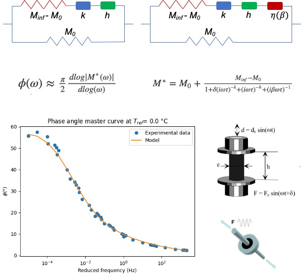
that, based on the relationship proposed by Booij & Thoone [2] \( \phi(\omega) \approx \frac{\pi}{2} \frac{dlog|M^*(\omega)|}{dlog(\omega)} \),
computes the shift factor (\( a_T \)) for each isotherms at a given reference temperature as follows:
\( log(a_{(T_i,T_{ref})}) = \frac{\pi}{2} \sum_{j=i}^{j=ref} \frac{log|M^*(T_j,\omega)|-log|M^*(T_{j+1},\omega)|}{\phi_{avr}^{T_j,T_{j+1}} (\omega)} \).
In this case, a smooth and continuous master curve is obtained through the horizontal displacements quantified
by the shift factors (\( a_T \)) of the experimentally measured isotherms. Then, the William, Landel, and Ferry (WLF)
equation ( \( a_{T_{ref}} (T) =10^{\frac{C_1 (T-T_{ref})}{C_2 +T-T_{ref}}} \) ) is used to model \( a_T \), thus enabling the construction of the master
curve at any reference temperature with the following equations: \( C_2^{ref}=C_2^{ref'}+T_{ref}-T_{ref'} \) and \( C_1^{ref}=\frac{C_1^{ref'} C_2^{ref'}}{C_2^{ref}} \)
(Please verify if the curves on the Black Space and Cole-Cole diagrams display a certain continuity between the isotherms,
thus ensuring the application of the Time-Temperature Superposition Principle (TTSP). After the calculation,
the phase angles of the complex modulus and phase angle are plotted and the data can be found in
the “OUTPUT / Master curve data” text field (by scrolling the column). You can copy the three generated columns data [reduce frequency (hz), \( |M^*(f,T)| \) (Pa)
and \( \phi \) (°)] and also save each graph in .png format by right clicking on each figure.
Model parameter identification
The general 2S2P1D model [3] is implemented as follow: \( M^*= M_0+ \frac{M_{inf}-M_0}{1+\delta (i \omega \tau)^{-k} + (i \omega \tau)^{-h} + (i \beta \omega \tau)^{-1} } \). The model parameters are found by scrolling the column where checkboxes right next to each one will allow to determine the parameters that will be considered during the optimization process. Then click on the “Model Identification” button to compute an optimal set of parameters with which the drawn curves best fit your rheological measurements. The fact that you choose which parameters will be considered, it allows also to try other rheological models for your curve fitting:
- Huet-Sayegh (uncheck "activate β" parameter): \( M^*= M_0+ \frac{M_{inf}-M_0}{1+\delta (i \omega \tau)^{-k} + (i \omega \tau)^{-h} } \)
- 1S2P1D (Set \( M_0=0 \) and then uncheck it): \( M^*= \frac{M_{inf}}{1+\delta (i \omega \tau)^{-k} + (i \omega \tau)^{-h} + (i \beta \omega \tau)^{-1} } \)
- Huet (Set \( M_0=0 \) then uncheck both M0 and "activate β" parameters): \( M^*= \frac{M_{inf}}{1+\delta (i \omega \tau)^{-k} + (i \omega \tau)^{-h} } \)
Store parameters
After the calculation, the rheological parameters can be found in the “OUPUT / Calculated parameters” by scrolling the column from where you can copy them. Please note that the three Arhenius parameters A0, A1 and A2 that is used to model \( \tau(T) \) in the Viscoroute software [4] are also given. You can also store the parameters in the database assosiated with the data you have process. Several set of parameter can be saved for one data set.
[1] Emmanuel Chailleux, Guy Ramond, Christian Such & Chantal de La Roche (2006) A mathematical-based master-curve construction method applied to complex modulus of bituminous materials Road Materials and Pavement Design, 7:sup1, 75-92, DOI: 10.1080/14680629.2006.9690059
[2] Booij, H. C., & Thoone, G. P. J. M. (1982). Generalization of Kramers-Kronig transforms and some approximations of relations between viscoelastic quantities. Rheologica Acta, 21(1), 15–24. https://doi.org/10.1007/BF01520701
[3] François Olard & Hervé Di Benedetto (2003) General “2S2P1D” Model and Relation Between the Linear Viscoelastic Behaviours of Bituminous Binders and Mixes, Road Materials and Pavement Design, 4:2, 185-224, DOI: 10.1080/14680629.2003.9689946
[4] O. Chupin, A. Chabot, J.-M. Piau, D. Duhamel, Influence of sliding interfaces on the response of a layered viscoelastic medium under a moving load, International Journal of Solids and Structures, Volume 47, Issues 25–26, 2010,Pages 3435-3446,ISSN 0020-7683